Infiltration Editor#
FLO-2D uses three infiltration method. Green_Ampt, SCS, and Horton infiltration data development is outlined in this section. The INFIL.DAT file contains the infiltration data. The data can be global (uniform) or spatially variable at the grid element resolution. Global data is applied uniformly to all grid elements and spatially variable data allows different parameters to be applied to individual cells or groups of cells. The different methods for setting up the data are defined below.
Green-Ampt#
The Green-Ampt infiltration editor can add global or spatially variable infiltration data to the INFIL.DAT file. The FLO-2D plugin uses 4 tools for processing Green-Ampt data.
Global Infiltration Editor
Green-Ampt Polygon Schematize
Green-Ampt Infiltration Calculator (FCDMC Method 1)
Green-Ampt Log Average Infiltration Calculator (Full Green-Ampt Calculator)
Green-Ampt SSURGO and OSM databases
Global Uniform Infiltration#
Global infiltration parameters set a uniform infiltration for the grid system.
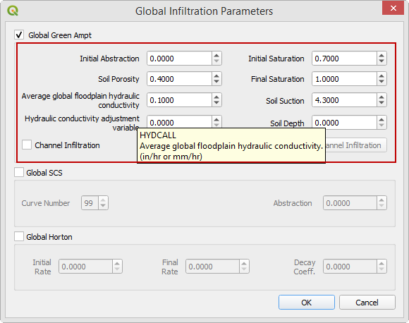
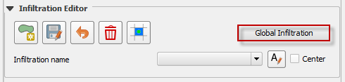
Global data is set up using the Global Infiltration button.
Click the button to open the editor dialog box.

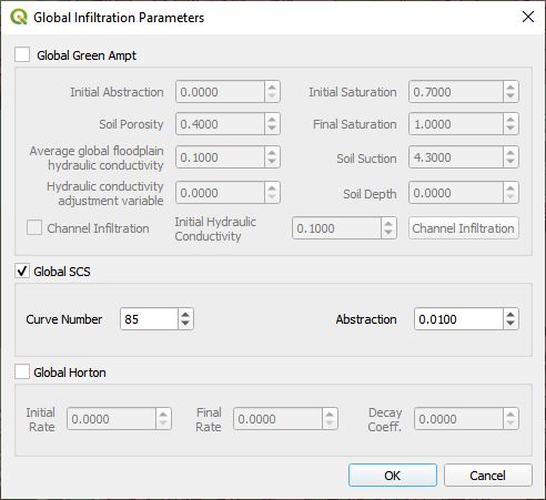
Check the Green-Ampt checkbox.
Fill the Green-Ampt with uniform infiltration parameters and click OK.
Tool tips have information related to the parameters. Hover the mouse pointer over the variable name to show the tooltip.
This option will set up uniform infiltration data for every grid element.
Spatial Infiltration Areas User Layer#
Simple polygon method#
Spatially variable floodplain infiltration is set by digitizing infiltration polygons into the Infiltration Areas user layer. Use the polygon editor to digitize spatially variable infiltration.
Create a polygon to represent an area of infiltration.
Click the create a polygon tool and digitize a polygon.
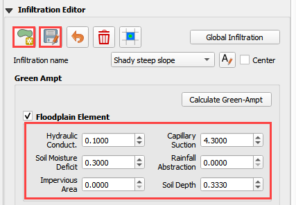
Name the infiltration polygon.
Fill the table for the infiltration data.
Click Save.
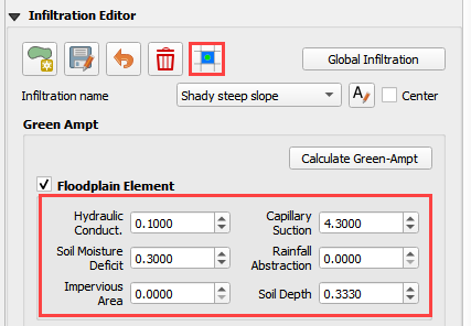
Fill the data in the widget for each new polygon.
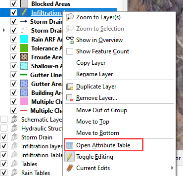
An alternate method to fill data to use the Attribute Table for the Infiltration User Layer.
Right click the layer and open the attribute table.
Click the Edit Pencil and start editing the data. Save and close the window.
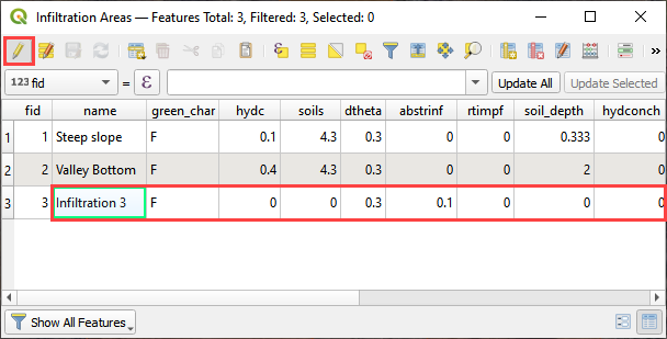
The data will automatically update in the widget.
Click the Schematize button to commit the changes to the grid.
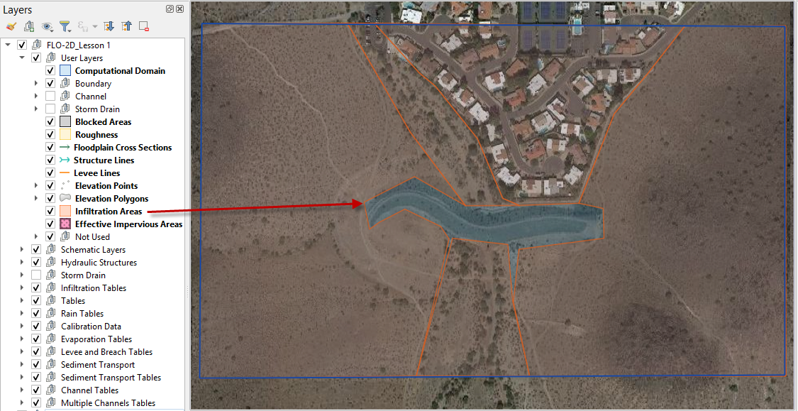
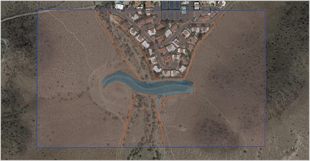
The infiltration polygons outline areas of cells that have similar infiltration characteristics. In the following image, the infiltration areas are different for urban, desert and desert drainage.
Channel Infiltration#
To assign channel infiltration, use the channel infiltration editor.
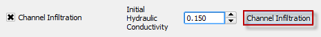
Set a global hydraulic conductivity for all channel elements.
Click the Channel Infiltration button.
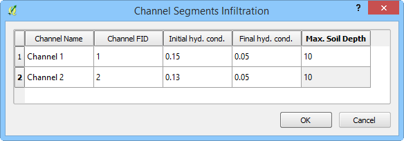
Local channel infiltration is set by segment in the dialog box.
Green-Ampt Infiltration Calculator FCDMC Method 2023#
To use the Flood Control District of Maricopa County (FCDMC) Green-Ampt calculator, the user must prepare or download soil, landuse, and eff shapefiles. The data maybe provided by the District. See the FCDMC hydrology manual for a more detailed discussion on modeling with the Green-Ampt method. Review the FLO-2D Plugin Technical Reference Manual for information pertaining to the Green-Ampt calculators. Review the FLO-2D Pro Reference Manual for information pertaining to the use of the Green-Ampt method by the FLO-2D engine.
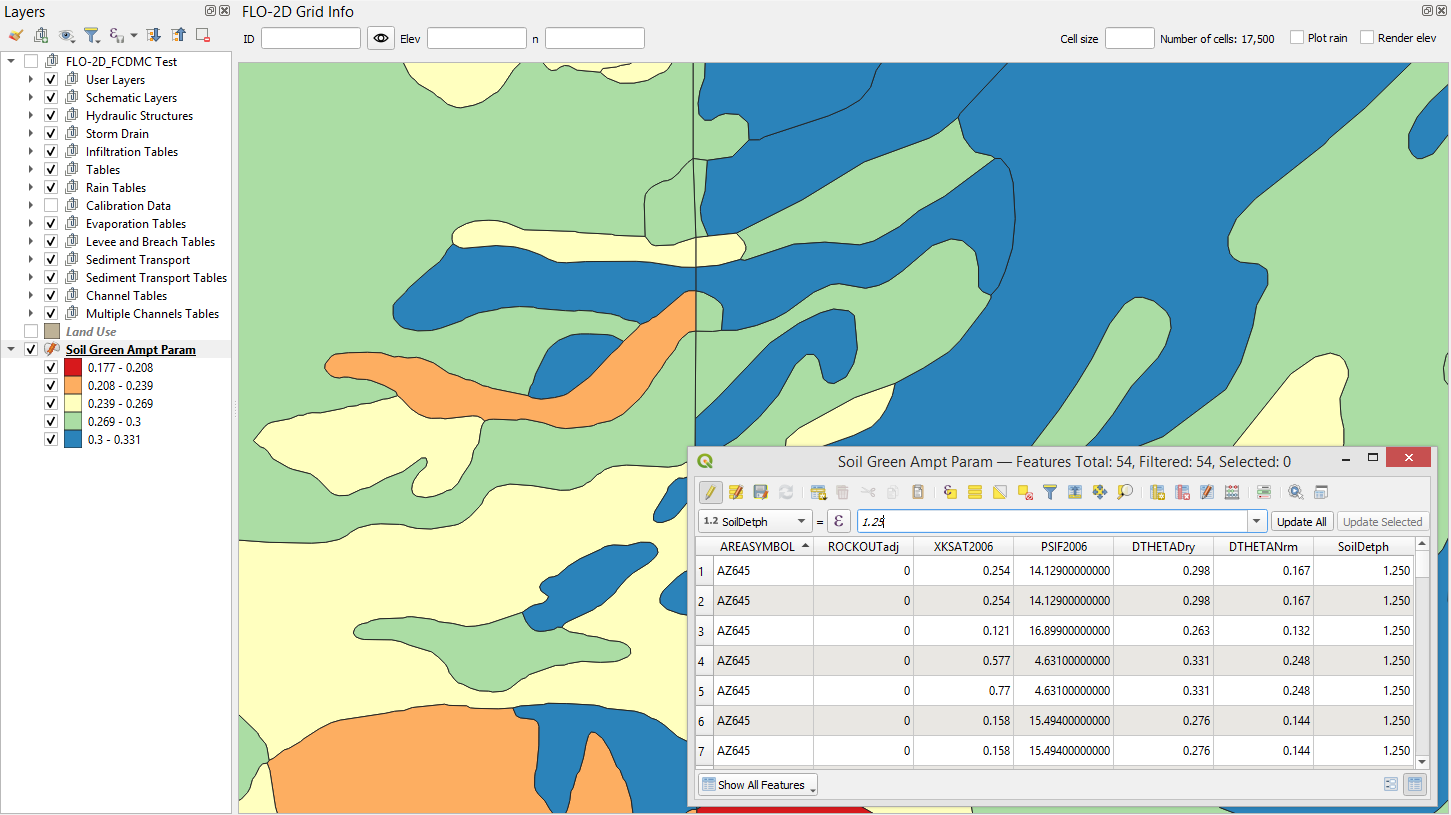
Prepare the soil data shapefile as seen in the following figure.
ROCKOUT is the percentage of rock outcrop coverage. 0 to 100
XKSAT is the hydraulic conductivity for the soil group. in/hr or mm/hr
Soil Depth is the limiting infiltration depth. Once the infiltration reaches this depth, it will turn off. ft or m
DTHETAdry is the soil moisture deficit for dry soil condition. It ranges in value from zero to the effective porosity.
DTHETAnormal is the soil moisture deficit for normal soil condition.
PSIF is the wetting front capillary suction. in or mm
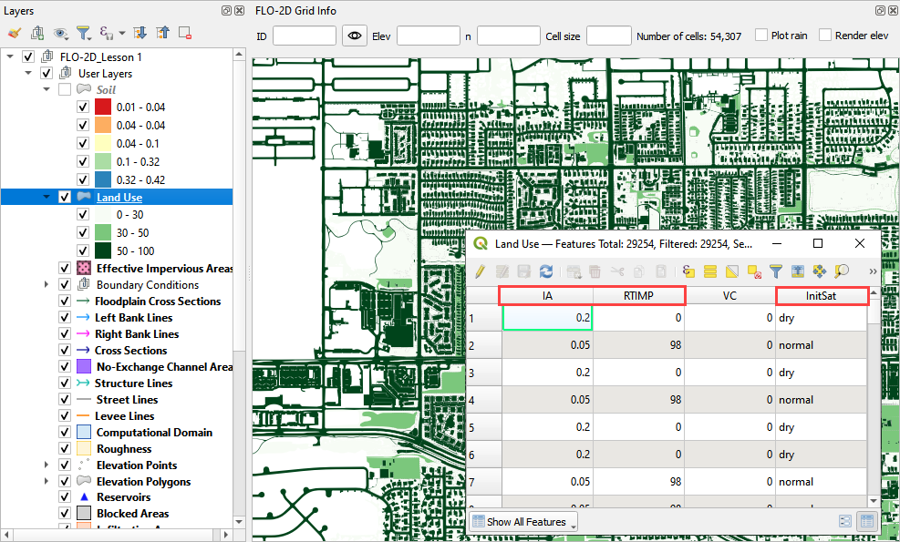
Prepare the Landuse data shapefile as seen in the following figure.
Saturation is the initial saturation condition. wet or saturated, dry, or normal
Initial Abstraction storage depth that must be reached before infiltration begins. in or mm
Impervious area is the percentage of impermeability for a given polygon. 0 to 100
Vegetative cover is not used by FCDMC. Leave it unchecked.
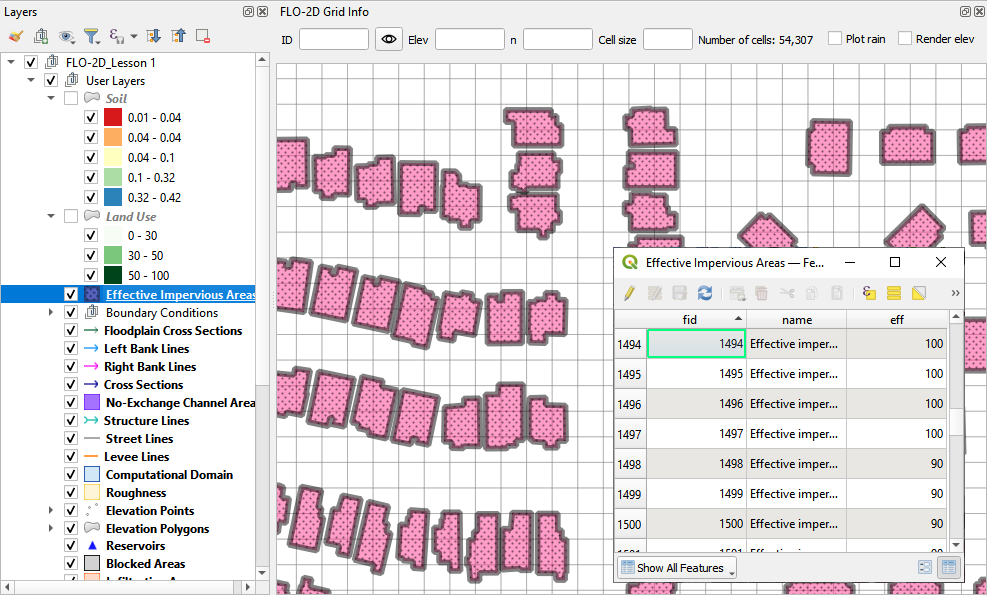
Prepare the EFF data shapefile as seen in the following figure.
Eff is the percent effectiveness of the impervious space. It pertains more to HEC-1 calculations but can also be applied as an additional control or adjustment for a 2D grid. If an EFF polygon is present, the calculator will multiply the RTIMPgrid * the EFF to determine a final RTIMP. 0 to 100
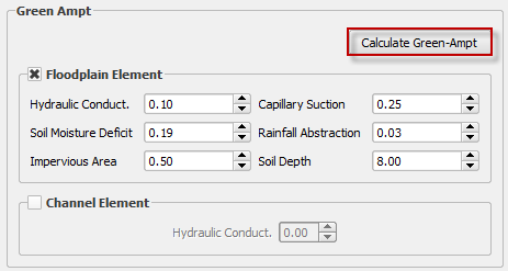
To run the calculator, click the Calculate Green-Ampt button.
Check if the User soil and landuse layer are selected, fill the form and click OK.
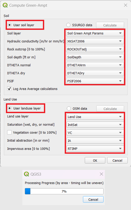
The calculator uses the calculation methods outlined in the FLO-2D Plugin Technical Reference manual.
When the infiltration calculator is finished, the following message will appear.
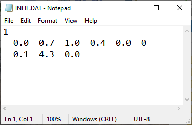
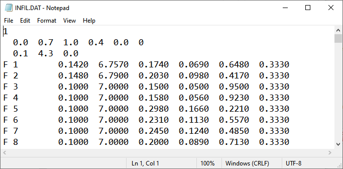
The INFIL.DAT file looks like this. For a detailed explanation of these variables, see the FLO-2D Data Input Manual INFIL.DAT section.
Green-Ampt SSURGO and OSM databases#
The user can estimate Green-Ampt parameters by leveraging data from two databases: the Soil Survey Geographic Database (SSURGO) and OpenStreetMap (OSM). The SSURGO database contains comprehensive information on soil, gathered through the collaborative efforts of the National Cooperative Soil Survey. Utilizing the NDOT Green and Ampt Rainfall Loss Parameters, the Green-Ampt parameters for different soil types can be estimated. This document outlines the methods and equations for developing Green and Ampt loss parameters for soils developed by Saxton and Rawls in 2006.
The OpenStreetMap (OSM) database, a freely accessible and continually updated geographic resource, relies on contributions from volunteers worldwide. This database provides data on land use, which serves as a component for estimating Green-Ampt parameters. In combination with the information available on the Drainage Design Manual for Maricopa County, estimations for Vegetation Cover, Initial Abstraction, and RTIMP can be determined for different land uses using the OSM dataset.
FLO-2D collects, organizes, and calculates the information from SSURGO and OSM databases. By preparing this data in shapefiles, it becomes readily available for use within the Green-Ampt calculator.
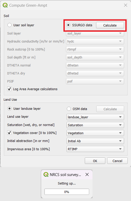
Select the SSURGO data and press calculate. This process downloads the data from NRCS and fills the missing data. Care should be taken because data could be scarce in some areas. Engineering judgment is essencial in such situations.
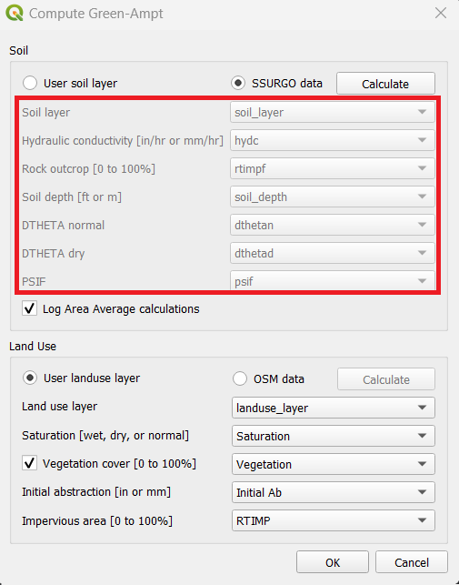
The soil layer and fields will be automatically updated once the process is finished.
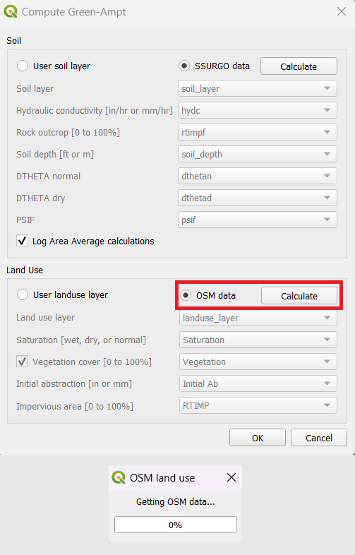
Select the OSM data and press calculate. This process downloads the data from OSM and generates the land use map. This process could take a long time for larger areas. This information is more precise in urban areas and less precise in rural areas. Engineering judgment is essencial for evaluating the data quality.
The landuse layer and fields will be automatically updated.
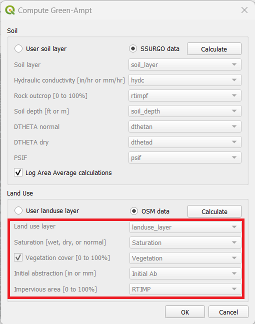
Check the form if the fields are correctly selected and click OK.
When the infiltration calculator is finished, the following message will appear.
The INFIL.DAT file looks like this. For a detailed explanation of these variables, see the FLO-2D Data Input Manual INFIL.DAT section.
SCS#
Global Uniform Infiltration#
The SCS infiltration editor can add global or spatially variable infiltration data to the INFIL.DAT file for infiltration curve numbers.
Set up the Global Infiltration first. Click Global Infiltration.
Fill the Global Infiltration dialog box.
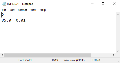
The INFIL.DAT file looks like this:
Where the infiltration type is 2 = SCS infiltration.
The 85 is the uniform curve number for each grid.
The 0.01 is the initial abstraction.
Spatial SCS Infiltration from Infiltration Areas User Layer#
Note
This method is the most effective way to sample SCS data. If using the other calculators, review SCS column for errors.
Spatially variable floodplain infiltration is set by digitizing infiltration polygons or importing infiltration polygons. Use the polygon editor to digitize spatially variable infiltration. Create a polygon to represent an area of infiltration.
Select the Infiltration Areas user layer.
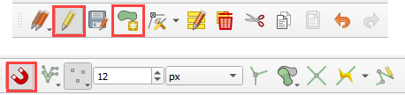
Click the editor pencil and snapping magnet button.
Create the polygons the represent areas with the same curve number.
Fill the table for the infiltration data.
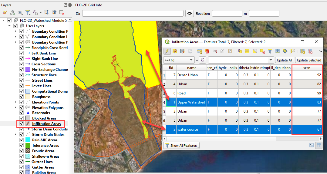
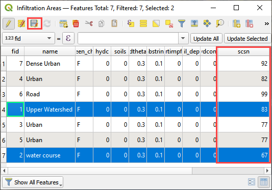
The finished table has a CN for every polygon.
Click the Save button to save the attributes.
Click the pencil button to close the editor.
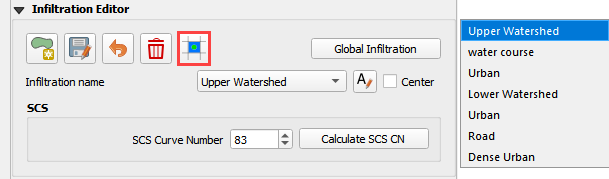
Check the data in the Infiltration Editor Widget. Click the Schematize button to complete the process.
The spatially variable INFIL.DAT looks like this:

Curve Number Generator#
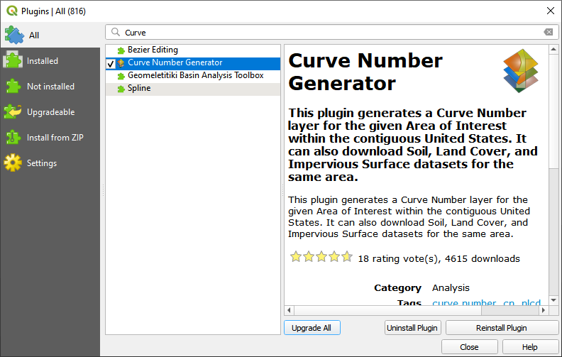
If necessary, add the Plugin Curve Number Generator.
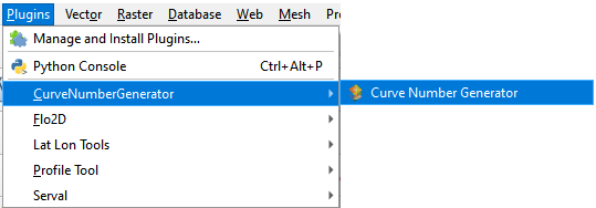
Open the Curve Number Generator.
Set the Area Boundary to the Grid. Check the boxes and click OK.
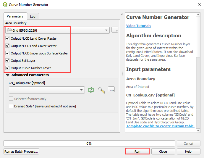
Click Close when process is finished. The Curve Number Polygon Layer can be used in the next section.
SCS Calculator From Single Shapefile#
Warning
If applying this method, review min and max of the SCS field. This method only works on polygon shapefiles that have no geometric deficiencies. If this method results in errors, copy the polygons to the User layer field and use the User Layer Method.
This option will add spatially variable infiltration data to the grid from a shapefile with one CN attribute field.
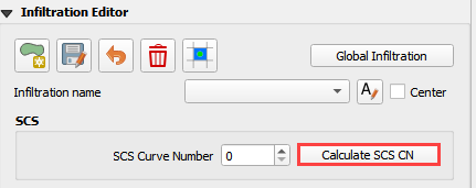
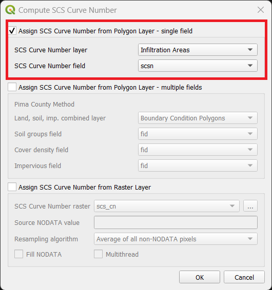
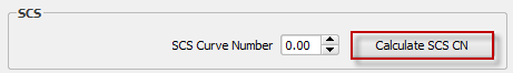
Click the Calculate SCS CN button.
Check the ‘Assign SCS Curve Number from Polygon Layer - single field’.
Select the layer and field with the infiltration data.
This method works for shapefiles that have a CN already calculated.
Click OK to calculate a spatially variable CN value for every grid element.
When the calculation is complete, the following box will appear. Click OK to close the box.
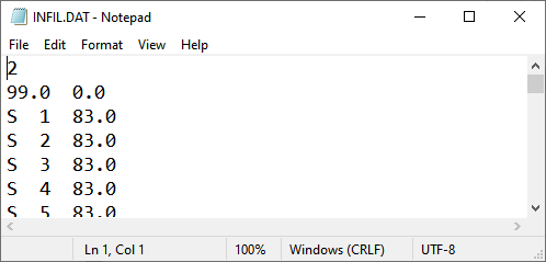
The INFIL.DAT file looks like this.
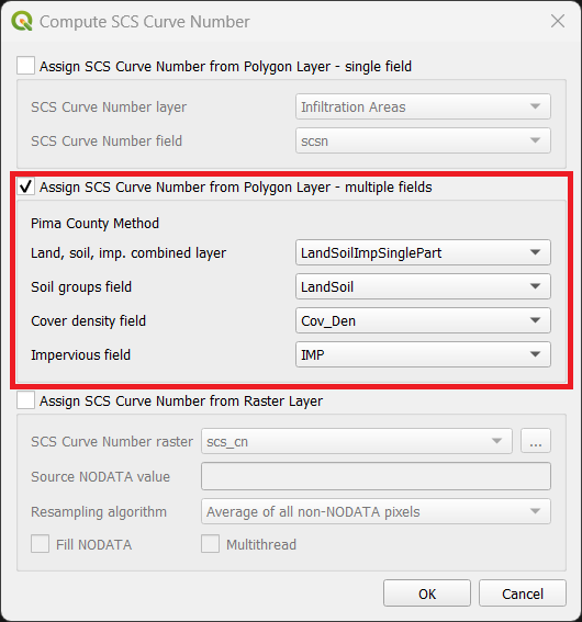
SCS Calculator From Single Shapefile Multiple Fields Pima County Method#
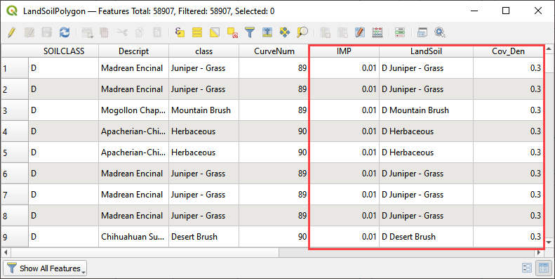
Use this option for Pima County to calculate SCS curve number data from a single layer with multiple fields. This is a vector layer with polygon features and field to define the landuse/soil group, vegetation coverage and impervious space. This option was developed specifically for Pima County.
The data should be arranged as shown in the attribute table.
Click the Calculate SCS CN button.
Check the ‘Assign SCS Curve Number from Polygon Layer - multiple fields’.
Select the layer and fields with the infiltration data and click OK to run the calculator.
When the calculation is complete, the following box will appear. Click OK to close the box.
The INFIL.DAT file looks like this.
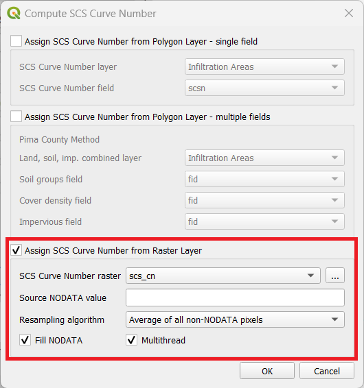
SCS Calculator From Raster Layer#
This option will add spatially variable infiltration data to the grid from a raster with cells containing CN values. Important properties:
The raster must have the same coordinate reference system (CRS) as the project. If the CRS is missing or is set by the user, save the raster with the correct CRS.
The best resolution of the grid element CN is achieved when the CN raster pixel size is smaller than the grid element size.
The raster warp method uses a weighted average to warp the original raster pixels to the cell size pixels.
Click the Calculate SCS CN button.
Check the ‘Assign SCS Curve Number from Raster Layer’.
Select the raster containing CN values from the dropdown or choose a raster from the file dialog.
Set the NODATA value.
Select the resampling algorithm.
Select the Fill NODATA option to set the CN of empty grid elements from neighbors. This is only necessary if there are empty raster pixels.
Select the multithread option to use all CPU’s for running the algorithm.
Click OK to calculate a spatially variable CN value for every grid element.
When the calculation is complete, the following box will appear. Click OK to close the box.
The INFIL.DAT file looks like this.
Horton#
Global Uniform Infiltration#
The Horton infiltration editor can add global or spatially variable infiltration data to the INFIL.DAT file for.
Set up the Global Infiltration first. Click Global Infiltration.
Fill the Global Infiltration dialog box.
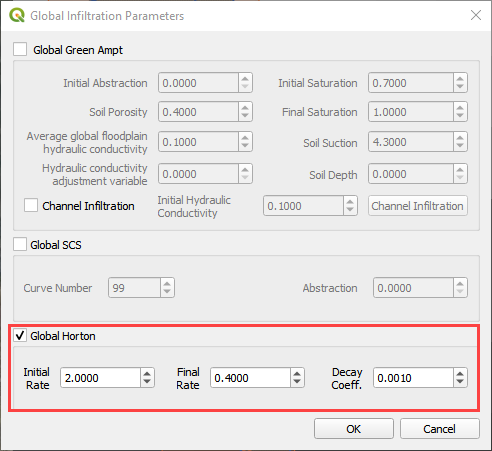
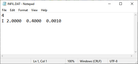
Uniform Horton infiltration is assigned as follows in the INFIL.DAT file:
Horton Spatially Variable Method#
Spatially variable Horton infiltration is created by digitizing infiltration polygons. Use the polygon editor to digitize spatially variable infiltration. Create a polygon to represent an area of infiltration.
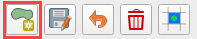
Click the create a polygon tool and digitize a polygon.
Click Save.
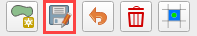
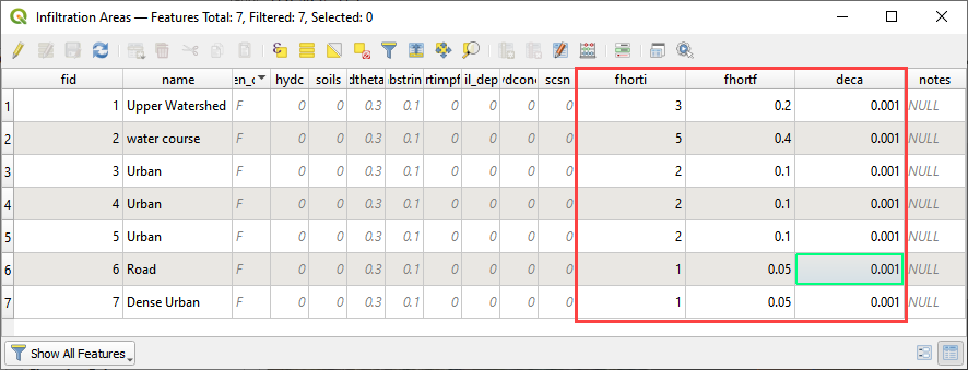
Right Click the Infiltration Areas layer (User Layers) and open the Attributes Table. Click the Editor Pencil button.
Name the infiltration polygons and fill out the data for fhorti, fhori, and deca.
Click the Save button and Editor Pencil button.
Click Schematize.
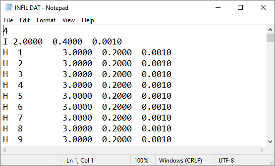
The spatially variable Horton looks like this in the INFIL.DAT file.
Troubleshooting#
Infiltration calculators all use intersection tools. This can cause problems if the shapefiles are not set up correctly. Specifically, land use and soils shapefiles that may have been converted from raster data. If errors persist, try “fix geometry”, “simplify”, and “dissolve” on the source shapefiles. These tools are part of the QGIS Processing Toolbox. They can also be corrected in ArcGIS if the datasets are very large.
Make sure the shapefiles completely cover the grid. If a grid element is outside the coverage of the infiltration, QGIS will show an error.
Make sure the shapefile fields have a correctly defined number type. The shapefiles that are supplied with the QGIS Lessons will help define the Field Variable Format such as string, whole number or decimal number.